

Dylan Lu1,*, Jan Hannig 1,2
Abstract
More than 50 years have passed since the Equal Pay Act of 1964, and women are still paid less than men. United States universities claim to be pioneers of social progress and so it is of interest to know whether the gender wage gap exists there. This study sheds light on the academic gender wage gap by comparing the salaries of male and female assistant professors within three years of being hired at selected U.S. public universities. The group of assistant professors are likely to satisfy our exchangeability assumption because early career faculty tend to come with similar experience. Finally, we focus on public university faculty because their salaries are publicly available. The data studied was collected from salary reports from public university systems in 2018 and 2019 under the Freedom of Information Act. Due to the novel way of assigning gender using genderize.io, traditional statistical methods for comparing two populations are not appropriate. For this reason, this study uses permutation-based non parametric tests that are valid for the data. Our study examines the presence of the gender wage gap in U.S. public universities and finds that significantly more women receive lower salaries than men. For example, the proportion of women making less than $10,000 a month is 12% higher than the proportion of men making the same amount. The study concludes that gender disparities within academic disciplines are a considerable factor contributing to the wage gap.
Introduction
The gender wage gap is commonly represented by the difference between the median earnings of male and female employees (Fontenot et al. 2018). More than five decades after the Equal Pay Act of 1964, the gender wage gap still exists. In 2017, women made only 80.5 cents for every dollar a man made (Fontenot et al. 2018). This wage gap is one of the factors that leads to poverty (Gradín et al. 2010). Women experience a higher rate of poverty than men. In 2019, 10.8% of women and 8.1% of men aged 18 to 64 lived in poverty. (Semega et al. 2019). Changes in family structure have amplified the problem. In the past 40 years, there has been a dramatic increase in breadwinner mothers, who participate in paid jobs and provide for their families. According to Glynn (2019), “In 2017, 41 percent of mothers were the sole or primary breadwinners of their families, earning at least half of their total household income.” The fact that women do not receive equal compensation has a significant impact on their entire families including their children (Gradín et al. 2010). For example, Gradín et al. (2010) claim that 10 percent of poor residents in Spain and Portugal could leave poverty if gender wage discrimination were to disappear.
Gender gaps in faculty salary have been studied extensively to understand the academic labor market. Economic models were applied to estimate human capital and con- trol for variables such as seniority, education, productiv- ity and experience. After controlling for faculty character- istics, female faculty members still make significantly less money than their male counterparts (Umbach 2007; Bar- bezat 2005; Toutkoushian 2005), though this gender wage gap has decreased since 1969 because of the Equal Pay Act of 1964 (Toutkoushian 2005). Academic discipline has been identified as a contributing factor because disciplines earning less money have a high proportion of female faculty (Umbach 2007; Perna 2001; Smart 1991). The assumption has been made that those disciplines with a large focus on science and engineering have a larger gender gap in faculty salary than other disciplines (Johnson and Taylor, 2019).
Dataset from previous studies came from the National Survey of Postsecondary Faculty (NSOPF:99), collected in 1999 (Umbach 2007; Barbezat 2005; Toutkoushian 2005), or from the Survey of Earned Doctorates (NSF), collected from 2003 to 2011 (Johnson and Taylor 2019). During the past 20 years, many fields such as data science and computer science have experienced substantial salary inflation due to competition from nonacademic employers, such as Microsoft, Google and Facebook. According to Umbach (2007), “It would be more pertinent to study current data in order to view the persisting effects in the current labor market.” In this manuscript, gender wage disparities were examined using current data collected in 2018 and 2019, which were the latest data available at the time this work was conducted.
Since the data were reported for every employee by their employers as opposed to being collected by voluntary surveys, this dataset does not suffer nonresponse bias. However, limited information about each employee makes explicitly accounting for individual performance measures, such as the effectiveness of teaching and research, difficult. This study focuses on assistant professors within three years of their hiring. Since all these early career faculty were recently hired through a competitive job search, it is assumed that they have roughly the same human capital, such as education, experience, and productivity, as other recent hires in their field (Larson et al. 2014). Initial salary differences persist due to the “annuity feature” of faculty salaries (Hearn 1999), i.e., annual faculty salary adjustments are typically a small percentage of the previous year’s salary (Hansen 1988). Thus, another reason to use early career faculty is to focus on current practices and remove potential legacy effects of discrimination that may have happened decades ago.
In previous studies, the effect of covariates was con- trolled using linear models (Umbach 2007; Barbezat 2005; Toutkoushian 2005) which may be overly simplistic because non-linear effects potentially exist. Additionally, because gerderize.io was used to predict gender based on first name (Genderize.io, 2021), many observations are partially assigned to both males and females, e.g., Erin is used as 77% female and 33% male, while Peter is 99% male and 1% female. This data does not satisfy the independence assumptions of statistical tests comparing two independent samples, such as Kolmogorov–Smirnov test (Smirnov 1939). Consequently, these traditional statistical tests cannot be used on this data. One of the novel aspects of this work is the use of permutation-based nonparametric statistical methods that are valid for this data. The main assumption of permu- tation tests is exchangeability, i.e. the members in the group being permuted should have roughly the same characteris- tics. This assumption is satisfied for early career faculty with similar human capitals (Larson et al. 2014).
Our work shows that the gender wage gap still persists among assistant professors in the U.S. public universities. Part of the observed gender wage gap can be explained by the fact that male dominated disciplines such as computer science or economics earn much higher salaries than disciplines with a higher proportion of women such as nursing. However, even accounting for this effect leaves some unexplained wage gaps. Thus, starting assistant professors should consult the publicly known information on current salary levels in their disciplines prior to negotiating compensation. Moreover, higher paying disciplines should find ways to encourage more women to become faculty.
Materials and Methods
Description of the Data
Since faculty salaries in public universities are a matter of public record, the latest salary information was obtained for several large public universities. In particular, the data studied included 87,260 employees from four university systems: the University of North Carolina System (UNC) in 2019, the University of Michigan System (UMich) in 2019, the University of Wisconsin System (UWisconsin) in 2018 and the Rutgers University System (RU) in 2018. These are the latest data available when the research was conducted. The annual inflation between 2018 and 2019 was low (2.44%), and, therefore, it does not affect the conclusion of the study (U.S Bureau of Labor Statistics, 2023).
The data were primarily collected online from databases provided by each university. The exception is the data from UMich, which was collected by contacting its Freedom of Information Act Office. The data include variables such as name, school, campus, department, title, service day and salary.
Inclusion/Exclusion Criteria
The data were filtered to include only faculty hired within the past three years. Visiting assistant professors, teaching assistant professors, and clinical assistant professors were excluded from data since the primary interest is in tenure- track assistant professors. Additionally, approximately 0.6% of cases (n = 21) were eliminated because of extremely low reported salaries, reported as less than 3,000permonth.ManypublicuniversitiesintheU.S.havesalarybandswithminimathatarefarhigherthan3,000 per month. For example the salary bands for the University of North Carolina at Charlotte (UNC Charlotte campus response 2021). Three faculty members randomly chosen out of the 21 were contacted, and they confirmed that their reported salary was a fraction of what they actually received. The number of employees at each university are documented in Table 1.
Table 1. Number of employees and assistant professors in each university systems. Only the data on assistant professors was used in this study.
School | Number of all employees | Number of assistant professors |
Total | 87,260 | 3,248 |
UNC | 48,710 | 1,640 |
RU | 4,327 | 519 |
UWisconsin | 30,601 | 644 |
UMich | 3,622 | 445 |
Data Cleaning
Because different schools use different ways to record salary information, monthly salaries were computed to make results comparable across universities. For example, the UNC system reports full-time equivalents (FTE) and employment months for each of its employees. FTE is a unit that indicates the workload of a faculty and is calculated as a faculty’s scheduled hours divided by the faculty’s hours for a full- time workweek. Employment month indicates the number of months a faculty member works during a year. Typically, this is nine or twelve months. The monthly salary is then computed by the formula:
monthly salary=salaryemployment months⋅FTE
The other schools do not report employment months; however, typical employment months are consistent within disciplines depending on the discipline culture. Therefore, we computed an average employment month for each discipline based on the UNC data and used this to compute monthly salary for all the other schools.
For Rutgers University, some faculty titles indicate the number of employment months. For example, the title “Assistant Professor Academic Year” implies that the number of employment months is 9, and “Assistant Professor Calendar Year” implies that the number of employment months is 12. Therefore, the monthly salary of these observations was computed based on this information.
Since the data do not provide gender information, the genderize.io API was used to predict gender based on first names (Genderize.io 2021). The “GenderGuesser” package (Caddigan 2015) was used to connect the API to R. The result contained a person’s predicted gender and the probability of being a male or female. Then, the data from the four schools were combined. Because the names of departments at various universities are different, a new label was created grouping departments together based on both the mean salary and the name of the department (Table 2).
This was stored in a variable called ”Discipline”. For example, electrical and computer engineering, information systems and computer science all belong to computer science, so they were combined. The final dataset contained 3,248 assistant professors and 10 variables: school, campus, name, title, department, discipline, gender, monthly salary, proportion of male, and proportion of female.
Table 2. A complete list of the aggregated disciplines and their mean employment month for controlling the disciplinary effects. The average employment month was computed for each discipline based on the UNC data.
Discipline | Number of Assistant Professors | Mean employment month | Mean month salary |
Agriculture | 39 | 11.36 | $ 7,424 |
Art and Design | 65 | 9.04 | $ 7,794 |
Biochemistry | 110 | 10.86 | $ 9,649 |
Biology | 100 | 9.6 | $ 7,629 |
Business | 334 | 9.38 | $ 13,818 |
Chemistry | 43 | 9.3 | $ 7,772 |
Communication | 80 | 9.45 | $ 7,143 |
Computer Science | 151 | 9.71 | $ 11,019 |
Criminal Justice | 39 | 9 | $ 7,336 |
Cultural Studies | 124 | 9.14 | $ 7,761 |
Dramatic Arts | 68 | 9.2 | $ 6,582 |
Economics | 54 | 9.05 | $ 13,400 |
Education | 144 | 9.43 | $ 7,499 |
Engineering | 126 | 9.44 | $ 9,664 |
English | 56 | 9.07 | $ 7,385 |
Environmental Science | 130 | 9.92 | $ 8,447 |
History | 50 | 9 | $ 7,593 |
Law | 16 | 10.5 | $ 13,536 |
Library | 19 | 10.82 | $ 8,045 |
Math | 130 | 9.24 | $ 7,495 |
Medicine | 622 | 11.95 | $ 14,973 |
Music | 60 | 8.97 | $ 7,279 |
Nursing | 99 | 9.94 | $ 8,753 |
Philosophy | 26 | 9 | $ 7,245 |
Physics | 52 | 9.35 | $ 8,368 |
Political Science | 68 | 9.17 | $ 8,849 |
Psychology | 112 | 9.34 | $ 7,872 |
Public Health | 79 | 10.39 | $ 8,477 |
Sociology | 133 | 9.36 | $ 8,194 |
Sport Science | 65 | 9.42 | $ 7,972 |
Statistics | 54 | 9.33 | $ 10,269 |
Statistical Analysis
The empirical cumulative distribution function (empirical CDF) was plotted to visualize the gender wage difference in the combined data from the four universities. Since gender was obtained by prediction, the empirical CDF was adjusted by the gender probabilities computed by genderize.io using first names. Each data point was weighted by its associated probability of being male or female. Those points with higher gender probabilities overshadowed others with low gender probabilities. Below are formulas for the male and female faculty salary empirical CDF,
Fn(t)male=∑nj=11{Zj≤t}pj∑nj=1pj
Fn(t)male=∑nj=11{Zj≤t}pj∑nj=1pj
where Zj's are the observed salaries, the indicator function I{Zj≤t} is either 1 if Zj≤t or 0 otherwise, pj is the proportion of males associated with the jth first name, and qj=1−pj is the proportion of females associated with this name.
The next question to answer is whether the difference between CDFs was statistically significant. To this end, a permutation test was used. In particular, a comparison was made between male and female empirical CDFs with the dif- ference of the empirical CDF, where the gender proportions pj and qj were randomly reassigned. Additionally, a sec- ond permutation test was devised to determine that the dif- ferences observed in the first test are not caused by different gender balances within various disciplines, and to avoid the Simpson’s Paradox (Blyth 1972). In particular, gender pro- portions were randomly reassigned among faculty only within their own disciplines (Table 2), i.e., biologists’ genders were replaced with those of other biologists, medical doctors’ gen- ders were replaced by those of other medical doctors, etc. In this case, only genders of faculty within the same discipline were permuted.
To measure the difference quantitatively, a p-value was computed that measures the probability that the mean of the random curve is smaller than the original curve. All points in the random curves and original curve were ranked, and the mean of the ranks for each curve was used to compute the p-value. In particular we, define a ‘1001 * nx‘ matrix:
A=(y0⋮y1000)=(a01⋯0.2a11⋯0.4⋮⋱⋮a1000,1⋯−0.3)
Entries in each row are the differences of male and female empirical CDFs for each curve. y0 denotes the original curve and y1,...,1000 denotes the permuted curves. Each of the ‘nx‘ columns corresponds to a different monthly salary where ‘nx‘ is the number of faculty. Next, we define a ‘1001 * nx‘ matrix:
T=(t01⋯2t11⋯3⋮⋱⋮t1000,1⋯1),
where the entries of T are the ranks of the entries of A within each column. We also define the row-wise mean as:
meani=1nxnx∑j=1tij.
Hence, the permutation p-value is then defined as,
p=proportion(mean0≥meani)=110011000∑i=0I{mean0≥meani}
Results
The number of employees at each university are documented (Table 1). Prevoisuly in Table 2, the aggregated disciplines were selected, and their mean salaries and mean employ- ment months were calculated. The empirical CDF for female faculty was above its male counterpart in the range between 6,310and25,119 per month (Figure 1).
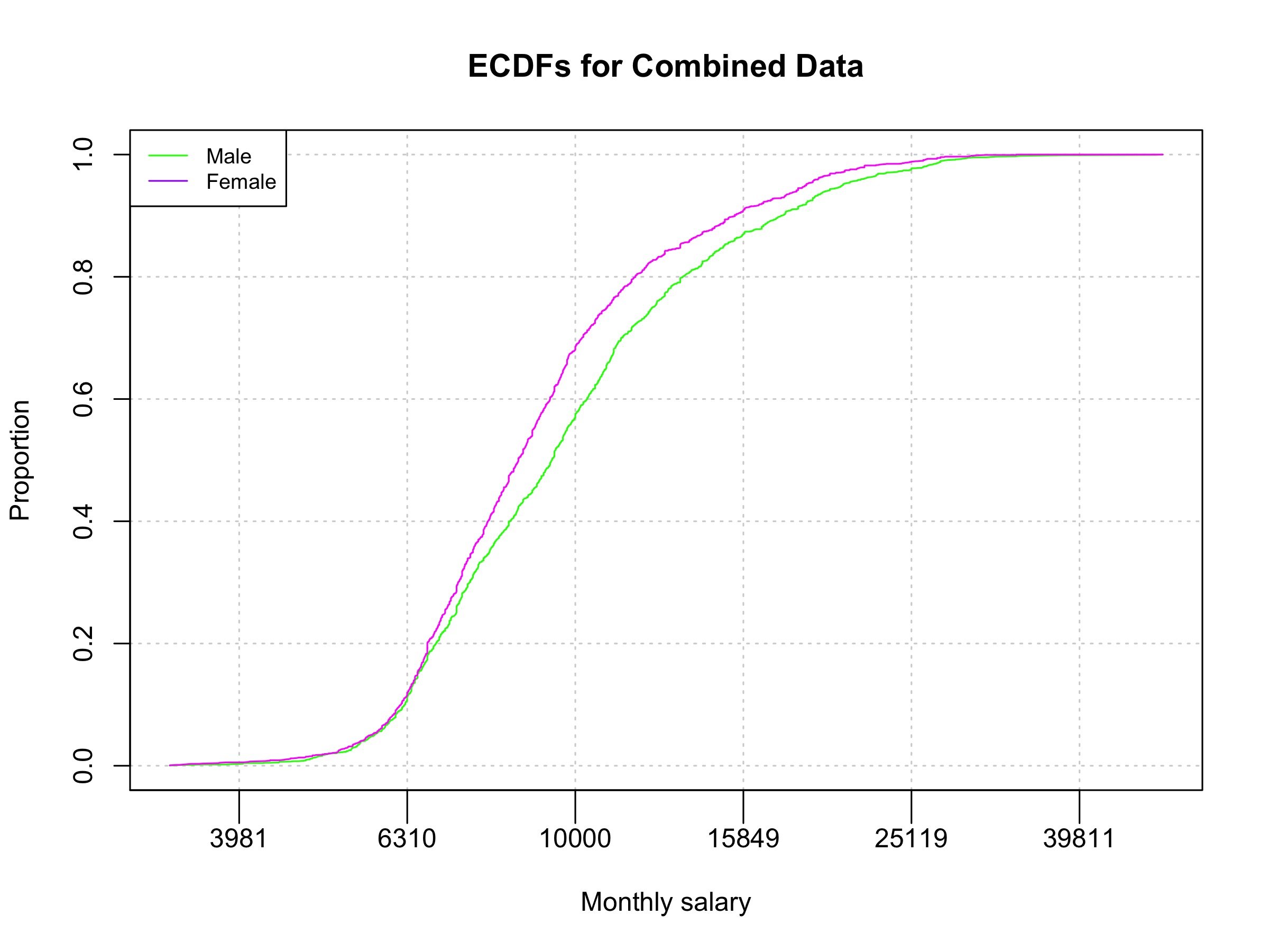
Figure 1. Empirical cumulative distribution functions contrasting the distribution of male and female salaries for combined data. On the x-axis is log10 of monthly salary. On the y-axis is the proportion of people in each group making less than the corresponding salary on x-axis.
After applying a permutation test on the entire population (not controlling for discipline), the non-permuted difference between male and female empirical CDFs (black curve) was far lower than the differences computed using the permuted population (blue envelope), which gives us a measure of what could be expected due to pure chance (Figure 2).

Figure 2. The difference of male and female empirical distribution functions (black line) for combined data compared to a thousand of differences with randomly assigned gender (blue lines). On the x-axis is log10 of monthly salary. On the y-axis is the proportion of males minus the proportion of females making less than the corresponding salary on x-axis
The corresponding permutation p-value is 1/1001. Next, after permuting faculty genders only within each discipline (controlling for discipline), the results show that the differ- ences of empirical CDFs based on genders permuted within discipline follow a similar pattern to the difference based on non-permuted data (Figure 3).
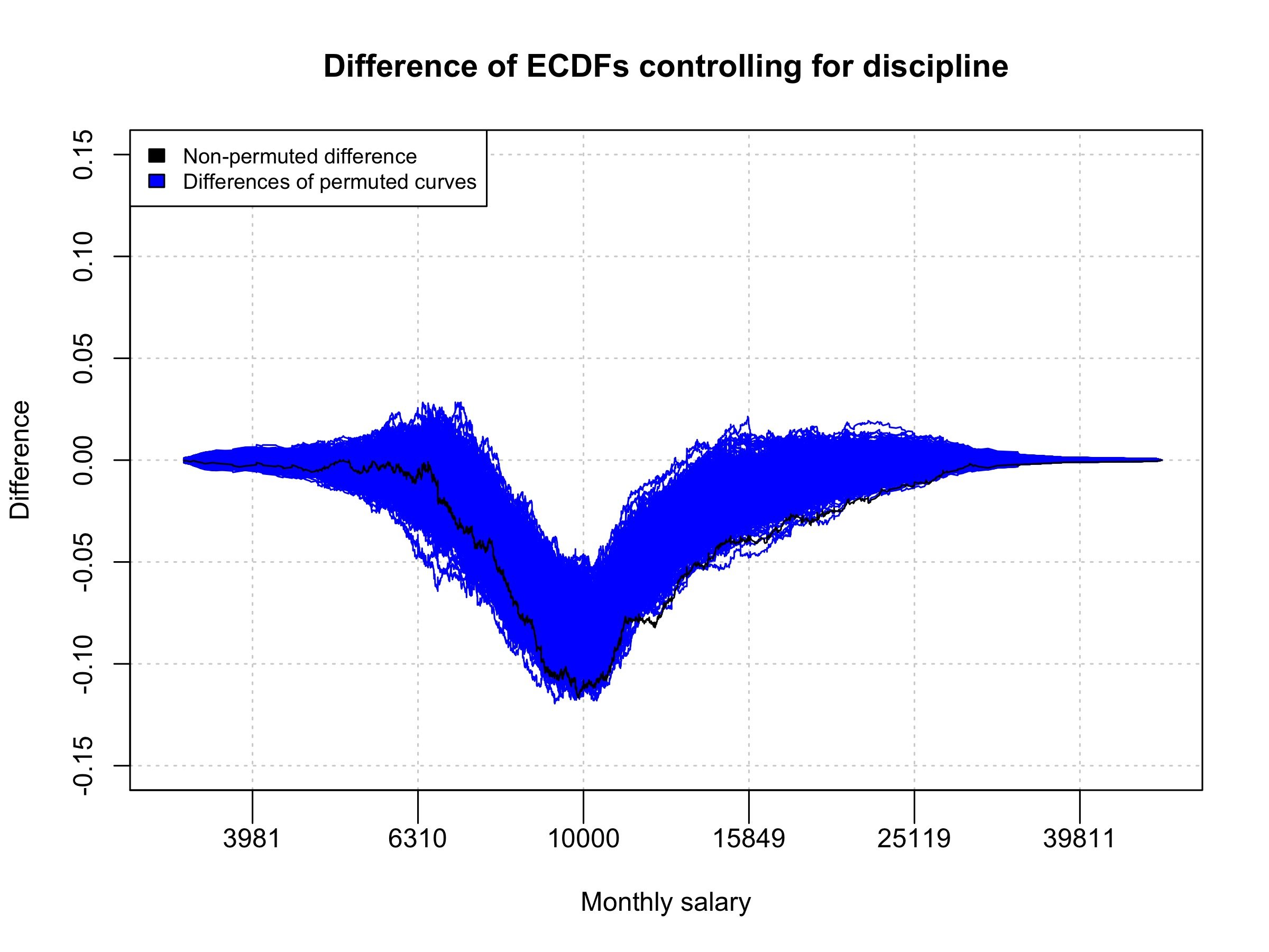
Figure 3. The difference of male and female empirical distribution functions (black line) for combined data compared to a thousand of differences with randomly assigned gender (blue lines). On the x-axis is log10 of monthly salary. On the y-axis is the proportion of males minus the proportion of females making less than the corresponding salary on x-axis.
After analyzing all schools together, each school was analyzed individually. P-values for the second permutation test (controlling for discipline) were computed (Table 3).
Table 3: p-values testing for existence of gender wage gaps accounting for discipline difference by university systems. The p-values used are the permutation p-values devised in the method section specifically for this model.
| p-value |
Combined Data | 0.017 |
UNC | 0.082 |
RU | 0.0011 |
UWisconsin | 0.170 |
UMich | 0.482 |
For Rutgers University, the p-value is less than the threshold of .05, while for the University of North Carolina, the p-value is less than .1. For these two universities, non- permuted differences remained near the bottom of the blue envelope, representing the differences of permuted curves (Figure 4).

Figure 4. The difference of male and female empirical distribution functions (black line) compared to a
thousand of permuted differences with randomly assign gender within discipline (blue lines) for each of the four university systems separately. On the x-axis is log10 of monthly salary. On the y-axis is the proportion of males minus the proportion of females making less than the corresponding salary on x-axis.
For the University of Wisconsin and the University of Michigan, the p-values were much greater than .1 and the non-permuted differences were well within the blue envelope (Figure 4).
Discussion
Through analysis, the empirical CDFs of males and females indicated that a gender wage gap clearly exists, the proportion of female faculty making less than the values in the x-axis was higher than the corresponding proportion of male faculty in the salary range between 6,310and25,119 per month (Figure 1). The most pronounced wage difference seems to be at approximately 10,000amonth,meaningthattheproportionofwomenmakinglessthan10,000 a month is 12% higher than the proportion of men making less than $10,000 a month. The wage difference is statistically significant as validated by a permutation p-value less than .001. Permutation tests also showed that most of the gender wage gap can be explained by discipline; namely, some disciplines have a high proportion of females while offering overall lower salaries. After accounting for disciplines, the gender wage gap becomes closer to a statistical error. The non-permuted difference was nearly contained in the differences of permuted curves (blue envelope). However, the non permuted difference tended to be on the lower edge of the blue envelope; therefore, there is still some wage difference that remains unexplained. The existence of some unexplained gender wage gap was confirmed by the fact that the p-value for the combined data was less than the threshold of .05 (Table 3).
For individual universities, the existence of unexplained wage gaps was present in the data from the Rutgers system (p-value < .05) but perhaps not present in the data from the Michigan and Wisconsin systems (p-value > .1). This result is unexpected and should be studied in more detail. Each system is made up of several different campuses, each with different Carnegie Classifications (The Carnegie Classification of Institutions of Higher Education 2021), e.g., doctorate granting universities, master’s colleges and baccalaureate universities. Therefore, the difference between systems may be due to either some policies specific to each university system or to different campuses having different pools of applicants. These would violate the assumption that all starting assistant professors have roughly the same human capital as other recent hires in their field.
One of the limitations of this work is that the nonparamet- ric approach does not allow us to quantify the size of the dis- ciplinary effect in dollars. Additionally, the method used can- not conclude causal relationships. Faculty salaries should be closely associated with individual performance; therefore, it would be valuable for future work to include performance factors such as the h-index and effectiveness of teaching in a nonparametric model. In addition, future research can integrate a survey together with the official salary report. How this information should be merged can be an interesting methodological challenge.
The phenomenon that women in some academic disci- plines opt out of their academic careers is described by a metaphor called the “leaky pipeline.” Women in academia have faced challenges such as sexism, maternity, family responsibilities and a glass ceiling. A recent study (Ysseldyk et al. 2019) showed that women holding postdoctoral posi- tions were more likely to experience stress and depres- sion and view themselves as less competitive than their male counterparts, especially in male-dominated science and engineering disciplines. A quantitative study associat- ing the change in percentage of women in BS, Ph.D. pro- grams and percentage of women among early-career faculty with gender wage gap may quantify the effect of the leaky pipeline.
Gender wage gap is one of the factors that leads to poverty (Gradín et al. 2010) and unfairly disadvantaged breadwinner mothers and their families (Glynn 2019). Thus, starting assistant professors should be well-advised to know their current salary levels in their disciplines when they are negotiating compensation packages. Similarly, university administrators should continue their efforts to reduce the gender wage gap and create a work environment conducive to family and life balance. Higher paying disciplines, such as science and engineering, should find ways to encourage women to become faculty and fix the leak in the academic pipeline.
In conclusion, even after 20 years of progress, conclu- sions of this study are broadly similar to those of past studies (Perna 2001; Toutkoushian 2005; Umbach 2007). There are clear gender wage differences and controlling for discipline explains some but not all of the differences.
References
Barbezat, D. and Hughes, J. (2005). Salary structure effects and the gender pay gap in academia. Research in Higher Education, vol 46, p621–640.
Blyth C. R. (1972). On Simpson’s paradox and the sure-thing principle. Journal of the American Statistical Association, vol 67 (338), p364–366. Available at: http: //dx.doi.org/10.2307/2284382.
Caddigan E (2015) GenderGuesser: Guess the gender of a name.
Gradín C., Coral D. R., and Olga C. (2010). Gender wage discrimination and poverty in the EU. Feminist Economics, vol 16:2, p73-109. Available at: http://dx. doi.org/10.1080/13545701003731831.
Genderize.io (2021). Genderize.io. Available at: https:/ /genderize.io (Accessed: 7 September 2021).
Glynn, S. J. (2019). Breadwinning mothers are increas- ingly the U.S. norm. Available at: https://www.americanprogress.org/article/breadwinning-mothers-continue-u -s-norm/ (Accessed: 18 Jan 2023).
Fontenot, K., Semega, J. and Kollar, M. (2018). Income and poverty in the United States: 2017. U.S. Census Bureau. Available at: https://www.census.gov/content /dam/Census/library/publications/2018/demo/p60 263.p df. (Accessed: 7 September 2021).
Hansen, L. (1988). Merit pay in structured and unstructured salary systems. Academe, vol 74(6) p10– 13. .
Hearn, J. C. (1999). Pay and performance in the university: an examination of faculty salaries. The Review of Higher Education, vol 22(4), p391-410. Available at: http://dx.doi.org/10.1353/rhe.1999.0016.
Johnson, J. A. and Taylor, B. J. (2019). Academic capitalism and the faculty salary gap. Innovative Higher Education, vol 44(1), p21-35.
Larson, R. C., Ghaffarzadegan, N. and Xue, Y. (2014). Too many phd graduates or too few academic job openings: the basic reproductive number R0 in academia. Syst Res Behav Sci., vol 31(6) p745-750. Available at: http://dx.doi.org/10.1002/sres.2210.
Perna, L. W. (2001). Sex differences in faculty salaries: a cohort analysis. The Review of Higher Education, vol 24 (3) p283-307. Available at: http://dx.doi.org/10.1353 /rhe.2001.0006.
Semega, J., Kollar, M., Shrider, E. A. and Creamer, J. (2019). Income and poverty in the United States.,. Retrieved from https://www.census.gov/
Smart, J. C. (1991). Gender equity in academic rank and salary. The Review of Higher Education, vol 14(4) p511–526.
Smirnov, N.V. (1939). Estimate of deviation between empirical distribution functions in two independent samples. Bull Moscow Univ., vol 2(2) (6.1, 6.2) p3–16.
The Carnegie Classification of Institutions of Higher Education (2021). About Carnegie Classification. Available at: https://carnegieclassifications.acenet.edu/ (Accessed: 18 Jan 2023). .
Toutkoushian, R. K. and Conley, V. M. (2005). Progress for women in academe, yet inequities persist: evidence from NSOPF:99. Research in Higher Education, vol 46 p1–28. .
Umbach, P. D. (2007). Gender equity in the academic labor market: An analysis of academic disciplines. Research in Higher Education, vol 48 p169–192..
UNC System Office Faculty Salary Ranges., (2021). Retrieved from https://provost.charlotte.edu/
U.S. Bureau of Labor Statistics (2023). CPI inflation cal- culator. Available at: https://www.bls.gov/ (Accessed: 31 March 2022).
Ysseldyk, R. Greenaway, K. H., Hassinger, E., Zutrauen, S., Lintz, J., Bhatia, M. P., Frye, M., Starkenburg, E. and Tai, V. (2019). A leak in the academic pipeline: identity and health among postdoctoral women. Front. Psychol., vol 10. Available at: https://doi.org/10.3389/fp syg.2019.01297.