
Authors: Alexandrea Churchill and Grace Kissling
Institution information: North Carolina State University, 121 Peele Hall, 10 Watauga Club Dr, Raleigh, NC 27607 National Institute of Environmental Health Sciences, 111 TW Alexander Dr, Durham, NC 27709
ABSTRACT
The National Toxicology Program (NTP) uses experimental designs which include exposing rodents to chemicals from in utero through two years of age. Each cohort consists of pups from various litters, suggesting that within-litter correlations should be considered when conducting statistical analyses as statistical significance of the dose-effect may be impacted by this litter effect. When the response under study, such as tumor occurrence, is a normally distributed continuous measure, to adjust for the within-litter correlation, a nested analysis of variance can be implemented. However, this is more difficult when the response is dichotomous and rare, such as the occurrence of less common tumors. When analyzing common tumors, within-litter correlations can be included into the mixed effects logistic regression models used to test for dose-effects. In contrast, when studying less common tumors, these models often fail to converge, and thus prevent testing for dose effects. The objective of this study is to determine the conditions under which mixed effects logistic regression models fail to converge using SAS procedures with litter correlations. These procedures were applied to datasets to evaluate the effects of the toxin AZT on tumors in mice and the effects of HMB on organ weights in rats. The p-values were examined to determine whether these endpoints were significantly related to dose. Overall, it was determined that when the dependent variable has a rare occurrence, optimization of the mixed model fitting cannot be completed and the tests for dose effects cannot be conducted. Therefore, future work should include research to determine which model should be used with a rare occurrence and how the analysis should be performed.
INTRODUCTION
Experimental designs used by the National Toxicology Program (NTP), such as exposing rodents to chemicals from in utero through two years of age, are conducted to learn more about the toxicity of substances in our environment (U.S. Department of Health and Human Services, 2013). A litter effect can be defined as the tendency for animals from the same litter to respond more alike than animals from different litters (Haseman and Kupper, 1979). Because natural litter-to-litter variation often exists, statistical significance of the dose-effect may be impacted by this litter effect (Lazic and Essioux, 2013). It is important to analyze data such that littermates are not assumed to be independent (Lazic and Essioux, 2013; OECD, 2007). As Bieler and Williams (1975) state, littermate correlation can have a huge impact on how toxicology data is modeled and analyzed. If within litter correlations are ignored, the effective sample size is overestimated, making the p-value smaller than it should be (Bieler and Williams, 1995). This could lead to significant results, when in fact, if within-litter correlations had been taken into account, the results would not have been significant. It has been previously reported that litter effects are a characteristic of dose response data and therefore, within-litter correlation must be included when conducting statistical analyses (Khera et al., 1989; Kupper et al., 1986). When the response is a continuous measure, adjusting for within-litter correlations is simple (Haseman and Kupper, 1979; Searle, 1971). To adjust for the within-litter correlation, when the continuous measure is normally distributed, a nested analysis of variance can be implemented (Haseman and Kupper, 1979). One paper states that adjusting for within-litter correlations is more difficult when the response is dichotomous and rare, such as the occurrence of less common tumors (Haseman and Kupper, 1979).
Different statistical models have been created to include litter effect, with many undergoing constant improvement (Yamamoto and Yanagimoto, 1994). Some models must be altered to incorporate litter effect, including the dose response model (Khera et al., 1989). Haseman and Soares (1976) concluded that, when analyzing experiments that look at dichotomous fetal responses, binomial or Poisson models provide poor fits, as there is similarity between responses from the same litter (Kupper et al., 1986). It also seems that certain models such as multistage, multihit and probit, which multiple authors have used, tend to ignore litter effects (Scientific Committee of the Food Safety Council, 1978, cited in Kupper et al., 1986; Segreti, and Munson, 1981; Kupper et al., 1986; Segreti, and Munson, 1981).
The beta-binomial model, considered by Williams (1975), is commonly used to account for littermate correlation when analyzing dose response data (Kupper et al., 1986; Khera et al., 1989; Yamamoto and Yanagimoto, 1994; Paul, 1982; Segreti and Munson, 1981). There have been a few concerns about using the beta-binomial model, such as difficulties with maximization (Tamura and Young, 1986; Khera et al., 1989; Bieler and Williams, 1995). Another possible model is the correlated probit model, which was proposed by Ochi and Prentice (1984) (Bieler and Williams, 1995; Yamamoto and Yanagimoto, 1994; Ochi and Prentice, 1984; Khera et al., 1989). However, this model is more complex compared to the beta-binomial model (Khera et al., 1989). Kupper and Haseman (1978) proposed the correlated binomial model (Yamamoto and Yanagimoto, 1994) while Bieler and Williams (1995) state that the quasi-likelihood approach is a very flexible method for including litter effect.
When using the logistic model and ignoring litter effects, there was typically no effect on the estimation of the parameters in the logistic model (Kupper et al., 1986; Khera et al., 1989). However, failing to take litter effect into account can cause significant underestimation of the true variances and can also lead to small confidence limits, as well as increased type I errors for test statistics (Kupper et al., 1986; Khera et al., 1989; Williams, 1975; Bieler, and Williams, 1995; Ochi and Prentice, 1984; Segreti and Munson, 1981). Even though the beta-binomial model is often used, it faces convergence issues when the dependent variable of interest, such as tumor presence, has a rare occurrence.
The statistical model used throughout this study is the mixed effects logistic regression model. This model includes fixed and random effects for the dichotomous dependent variable, along with covariates such as survival time and a cluster identifier to account for clusters - both additions which were necessary to incorporate into the model during this study. When analyzing common tumors, within-litter correlations can be included into mixed effects logistic regression models to test for dose-effects. However, when studying less common tumors, convergence problems with these models prevent testing for dose-effects. The objective in this study is to determine the conditions under which mixed effects logistic regression models fail.
MATERIALS AND METHODS
Using the statistical software SAS, we used SAS procedures for mixed effects logistic regression modeling to include litter correlations, such as PROC NLMIXED, PROC MIXED, and PROC LOGISTIC (SAS Institute Inc., 2009). The mixed effects logistic regression model used includes both fixed and random effects for a dichotomous dependent variable. This model assumes independence and normality of the random effects. PROC NLMIXED is used to fit nonlinear mixed models (SAS Institute Inc., 2009). PROC MIXED is used to fit mixed linear models to data, and enables these models to make statistical inferences about the data (SAS Institute Inc., 2009). PROC LOGISTIC fits linear logistic regression models for discrete response data by using the method of maximum likelihood (SAS Institute Inc., 2009). The statistical significance in tests for dose-effect was the primary outcome of interest. These procedures were applied to various types of data sets, such as the effects of 3’-azido-3’-deoxythymidine (AZT) on tumors in mice and the effects of HMB (2-hydroxy-4-methoxybenzophenone) on organ weights in rats (U.S. Department of Health and Human Services, 2006; U.S. Department of Health and Human Services, 2017). The p-values from these tests were then examined using tests of significance to determine whether these endpoints were significantly related to dose and whether there were significant litter effects, at a significance level of 0.05.
AZT Tumors
AZT is a known agent for the treatment of those with immune deficiency syndrome (AIDS) or seropositive for human immunodeficiency virus (HIV) and it is also known to cause cancer in mice born to mothers that are exposed to doses of 400 milligrams per kilogram of body weight or higher during their pregnancy (U.S. Department of Health and Human Services, 2006). In this specific study, female mice were exposed to lower concentrations of AZT (50 to 300mg AZT/kg body weight), both before and during their pregnancy in order to determine if the doses caused cancer in their offspring (U.S. Department of Health and Human Services, 2006). The mice used in this study were obtained from Charles River Laboratories, Raleigh, NC (U.S. Department of Health and Human Services, 2006). In the AZT tumors datasets, specific tumor types were evaluated separately as well as combined tumors in lung, liver, or skin. The AZT tumors datasets included the following variables: Dam, Sire, Dose (mg/kg/day), Sex (M/F), F1 pup, Lung-Alv/Bron Adenoma (X for occurrence), Lung-Alv/Bron Carcinoma (X for occurrence), Liver-Hepatic Adenoma (X for occurrence), Skin-Ulcer (X for occurrence), and survival days. The models carried out on the AZT tumors datasets included survival time as a covariate, and sire was used as the cluster identifier. P-values for the litter correlations were examined along with the estimates p-values of the other parameters, at a significance level of 0.05.
Beta-Hydroxy-Beta-Methylbutyrate (HMB) Organ Weights
The organ weight dataset was investigated to determine if the weights of any organs were affected due to the dose of beta-hydroxy-beta-methylbutyrate (HMB) in males by comparing only those in the same age group, while taking possible littermate correlations into account. Beta-hydroxy-beta-methylbutyrate is an ultraviolet absorbing compound. The HMB dataset included the following variables: Dose (ppm), TrtGrp (the treatment group for the rats), AnmID (animal ID), Sex (Male/Female), DamID, OrganName and OrganValue (organ weight). There were four dosage groups, 0 ppm (control), 1000 ppm, 3000 ppm and 6000 ppm. Females were removed from the analysis, as there was only one female pup per litter, so litter effects could not be estimated. Age was separated into two categories, group 1 included rats with postnatal days 110-114 and group 2 included rats with postnatal days 160-167. Harlan Sprague-Dawley rats were used in this study. Organ weights are continuous variables and were assumed to be normally distributed. The dataset was further investigated to determine which of the three dose groups differed from the control group and how they differed as well as looking at littermate correlation significance, all using a significance level of 0.05.
Hypothetical Datasets

Table 1. Display of the hypothetical dataset of litter size 12 consisting of 4 pups.

Table 1 (continued). Display of the hypothetical dataset of litter size 12 consisting of 4 pups each appears.
In addition, hypothetical datasets were generated and manipulated to look at the effects of litter size, number of pups, and percentage of pups affected. The datasets were created to determine if any of these variables mentioned had an effect on treatment group and littermate correlation significance. Hypothetical datasets were critical to investigate the differences between what was hypothesized and what was actually collected during the study. The initial hypothetical dataset was comprised of 12 litters, each containing four pups. The control group consisted of all unaffected pups i.e., a 0% tumor rate (later three of the zeros were changed to ones in order to get the model to run, as it would not work with all zeros). The treated groups had a 25% tumor rate in the pups, i.e., 25% of the group was one, the remainder was zero. In this data, a one indicates presence of a tumor, and a zero indicates absence of a tumor. The first treatment group consisted of a single one and three zeros in each litter. The second treatment group consisted of 50% of the litters having two ones and two zeros with the other 50% comprised of all four zeros. The third treatment group consisted of four litters containing three ones and one zero, and eight litters with all four zeros. The fourth treatment group consisted of three litters with all four ones and nine litters with all four zeros. A sample of this specific dataset can be seen in Table 1. Hypothetical datasets were also created for 24, 36, and 48 litters per group, with litter sizes of two, six, and eight pups. This concept was then applied to 12.5% of the pups being affected and later to 50% of the pups being affected. The mixed effects logistic regression model was used to obtain the parameter estimates and their p-values. The objective of this scenario was to determine which combinations of litter size and pups were significant for each percentage (%) group of pups affected. Graphs were produced to further examine these results.
RESULTS
AZT Tumors
Results from the analyses of the AZT tumors datasets indicated that littermate interactions were not significant for all tumor types investigated, i.e. lung, liver, and skin. Tables 2A-B and 3A-D illustrate these results. It was also found that when the tumor occurrence was low, the optimization of the model could not be completed. For females, the skin tumor model failed to converge with less than 10 tumors for all doses. For males, the liver tumor model failed with less than 20 tumors for all doses. The AZT tumors datasets look at both sire and dam as identifiers.

Table 2A. Model summary results for females in the AZT tumors example dataset. The significant values are highlighted in yellow. Pr > | t | is the probability that a greater absolute value of t, under the null hypothesis, is observed. s2u refers to the variance of the random effect u. * No values produced as optimization could not be completed.

Table 2B. Model summary results for males in the AZT tumors example dataset. The significant values are highlighted in yellow. Pr > | t | is the probability that a greater absolute value of t, under the null hypothesis, is observed. s2u refers to the variance of the random effect u. * No values produced as optimization could not be completed.

Table 3A. Display of the model summary results for females with the dam of the identifier for the AZT tumors dataset. The significant p-values are highlighted in yellow. Pr > | t | is the probability that a greater absolute value of t, under the null hypothesis, is observed. s2u refers to the variance of the random effect u.

Table 3B. Display of the model summary results for males with the dam of the identifier for the AZT tumors dataset. The significant p-values are highlighted in yellow. Pr > | t | is the probability that a greater absolute value of t, under the null hypothesis, is observed. s2u refers to the variance of the random effect u.

Table 3C. Display of the model summary results for females with the sire of the identifier for the AZT tumors dataset. The significant p-values are highlighted in yellow. Pr > | t | is the probability that a greater absolute value of t, under the null hypothesis, is observed. s2u refers to the variance of the random effect u.

Table 3D. Display of the model summary results for males with the sire of the identifier for the AZT tumors dataset. The significant p-values are highlighted in yellow. Pr > | t | is the probability that a greater absolute value of t, under the null hypothesis, is observed. s2u refers to the variance of the random effect u.
Beta-Hydoxy-Beta-Methylbutyrate (HMB) Organ Weights

Table 4. Display of the summary model results of the organ weight dataset. The significant p-values are highlighted in yellow. Pr > | t | is the probability that a greater absolute value of t, under the null hypothesis, is observed.

Table 5. Display of the differences of least squares means results from the organ weight data. The significant p-values are highlighted in yellow. Pr > | t | is the probability that a greater absolute value of t, under the null hypothesis, is observed.
For the HMB organ weight data, among males in age group 1 (postnatal days 110-114 age), terminal bodyweight was found to be significant (p = 0.0203) and among age group 2 (postnatal days 160-167), dorsal prostate weight (p = .0012), paired seminal vesicles (p = 0.0005), and terminal bodyweight (p = < 0.0001) were found to be significant. These results for the HMB organ weight dataset are illustrated in Table 4. After further investigation, it was determined that dorsal prostate weight in the 3000 ppm group was increased compared to the control, paired seminal vesicles weight in the 3000 ppm and 6000 ppm groups were both increased compared to the control and terminal bodyweight in the 6000 ppm group was decreased compared to the control. Terminal bodyweight in age group 1 was originally found to be significant at a significance level of 0.05, however when further investigated, it was found that the overall p-value for dose effect was 0.056. Although, the control vs 6000 dose group p-value was found to be significant (p = 0.0257). It was also discovered that littermate correlations were only significant for the terminal bodyweight for both age group 1 (p = 0.0376) and age group 2 (p = 0.0069). These results are shown in Table 5. The adjusted means, which take into account litter effects, with standard error bars for these three significant groups are presented in Figures 1A-D.

Figures 1A-D. Means with standard error bars as a function of dose, for each of the three significant organs. A) Dorsal prostate weight for males in age group 2.B) Paired seminal vesicles weight for males in age group 2. C) Terminal body weight for males in age group 1. D) Terminal body weight for males in age group 1.
Hypothetical Datasets
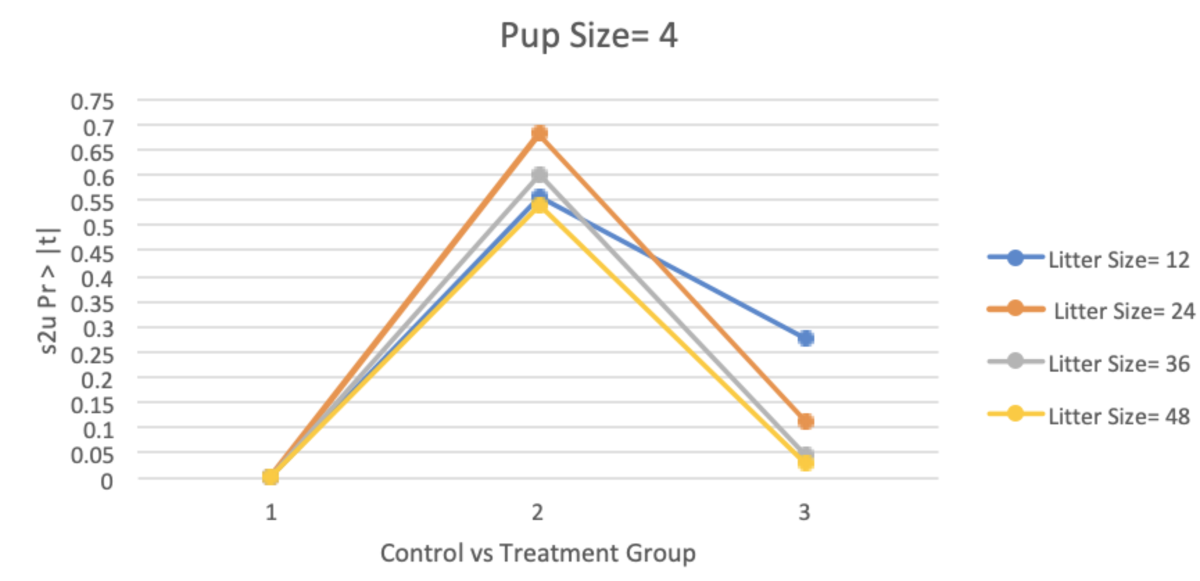
The overall summary of the hypothetical dataset format can be seen in Table 6. When looking at the results from the variations of the hypothetical data, it was reported that the p-values for littermate correlation between the control group and treatment group 1 (one tumor per litter) were almost always missing, indicating a failure of the SAS procedure to estimate littermate correlation in the model. This was because there were issues with convergence of the models. It was also shown that when only 50% of the litter was affected (12.5% tumor rate in pups) none of the p-values for the littermate correlation were significant at a significance level of 0.05; with litter size of 48, each consisting of four pups for control vs. treatment 3 being the closest (p = 0.0532).When treated groups had a 25% tumor rate in pups, the littermate correlation was found to be significant for seven multiple scenarios: 1) Litter size of 36 with four control pups vs. treatment 4 (p = 0.0416), 2) Litter size of 48 with four control pups vs. treatment 3 (p = 0.0480), 3) Litter size of 48 with four control pups vs. treatment 4 (p = 0.0218), 4) Litter size of 36 with six control pups vs. treatment 4 (p = 0.0487), 5) Litter size of 36 with six control pups vs. treatment 6 (p = 0.0409), 6) Litter size of 48 with six control pups vs. treatment 4 (p = 0.0268), 7) Litter size of 48 with six control pups vs. treatment 6 (p = 0.0230). When treated groups had 50% tumor rate in pups, the littermate correlation was found to be significant for five scenarios: 1) Litter size of 36 with four control pups vs. treatment 3 (p = 0.0448), 2) Litter size of 48 with four control pups vs. treatment 3 (p = 0.0274), 3) Litter size of 36 with six control pups vs. treatment 4 (p = 0.0263), 4) Litter size of 48 with 6 control pups vs. treatment 3 (p = 0.0391), and 5) Litter size of 48 with 6 control pups vs. treatment 4 (p = 0.0126). These overall summary model results are illustrated in Table 7. Tables 8A and B illustrate the finding that the litter size of eight did not show as many litter effects compared to a litter size of six. The p-values for littermate correlation almost always decreased from [control vs. single affected pup per litter] to [control vs. all affected pups per litter] (see Figure 2A for an example). However, the overall decrease was typically not linear, but instead consisted of various increases and decreases in p-values, see Figure 2B.

Table 6. Display of the hypothetical dataset format.

Table 6 (continued). Display of the hypothetical dataset format.

Table 6 (continued). Display of the hypothetical dataset format.

Table 6 (continued). Display of the hypothetical dataset format.

Table 7. Display of the model summary results for the hypothetical datasets. The significant p-values are highlighted in yellow. s2u refers to the variance of the random effect u.

Table 7 (continued). Display of the model summary results for the hypothetical datasets. The significant p-values are highlighted in yellow. s2u refers to the variance of the random effect u.

Table 7 (continued). Display of the model summary results for the hypothetical datasets. The significant p-values are highlighted in yellow. s2u refers to the variance of the random effect u.

Table 7 (continued). Display of the model summary results for the hypothetical datasets. The significant p-values are highlighted in yellow. s2u refers to the variance of the random effect u.

Table 7 (continued). Display of the model summary results for the hypothetical datasets. The significant p-values are highlighted in yellow. s2u refers to the variance of the random effect u.

Table 7 (continued). Display of the model summary results for the hypothetical datasets. The significant p-values are highlighted in yellow. s2u refers to the variance of the random effect u.

Table 8A. Display of the results from the mixed effects logistic regression modeling of the hypothetical dataset with 25% of the pups being affected per group. Litter size is 48 with 6 pups per litter. The significant p-values are highlighted in yellow. b0 is the intercept; Pr > | t | is the probability that a greater absolute value of t, under the null hypothesis, is observed. s2u refers to the variance of the random effect u.

Table 8B. Display of the results from the mixed effects logistic regression modeling of the hypothetical dataset with 25% of the pups being affected per group. Litter size is 48 with 6 pups per litter. The significant p-values are highlighted in yellow. b0 is the intercept; Pr > | t | is the probability that a greater absolute value of t, under the null hypothesis, is observed. s2u refers to the variance of the random effect u.

Figure 2. The relationships between the control and the treatment groups and their littermate correlation p-value. A) Results from the mixed effects logistic regression modeling of the hypothetical dataset with 50% of the pups being affected per group with 4 pups per litter. B) Results from the mixed effects logistic regression modeling of the hypothetical dataset with 25% of the pups being affected per group with 6 pups per litter.
DISCUSSION
Overall, it is important to include littermate correlations in the model when testing for dose effects when the littermates come from various litters (Lazic and Essioux, 2013). Several other studies, specifically a study conducted by Lazic and Essioux (2013) and a study on rabbits conducted by Gümüş et al. (2018), have stated the importance of taking litter effects into account. If within litter correlations had been ignored in this study then the resulting p-value may have been smaller than it should have been. This could have led to significant results which in truth may not have been significant if within-litter correlations had been taken into account, i.e. a Type I error. Furthermore, when the dependent variable of interest, tumor presence, has a rare occurrence, optimization of the SAS model fitting routines cannot be completed. Since most of the tumors in rodents are rare, the optimization of the mixed model fitting can occur on many of the tumor types in the experiment.
The objective of this study was to determine the conditions in which mixed effects logistic regression models fail to converge. For the AZT tumors and combined AZT tumors datasets, it was determined that the littermate correlations were not significant and therefore, the littermates can be modeled as independent. For the HMB organ weight dataset, it was determined that 1) dorsal prostate weight in the 3000 ppm group was increased compared to the control, 2) paired seminal vesicles weight in the 3000 ppm and 6000 ppm groups were both increased compared to the control, and 3) terminal bodyweight in the 6000 ppm group was deceased compared to the control. This is important as it gives insight into the effect of HMB on the weight of selected organs. It is hypothesized that the 3000 ppm and 6000 ppm dosage groups for the specific organ weights mentioned above increased due to the fact that HMB’s purpose is to protect muscle tissue. Littermate correlations were only significant at a significance level of 0.05, for the terminal bodyweight for both age groups 1 and 2. It was also reported that for the hypothetical datasets, the p-values for littermate correlation between the control group and treatment group 1 (one tumor per litter), were almost always missing, indicating a failure to estimate littermate correlation in the model. The p-values for littermate correlation almost always decreased from [control vs single affected pup per litter] to [control vs all affected pups per litter].
More work on this particular topic of rare occurrence of the dependent variable and the mixed effects logistic regression models failing to converge needs to be done in the field. Therefore, future research would potentially determine which model should then be used with a rare occurrence and how the analysis should be carried. This could include investigating and analyzing a variety of other datasets with dependent variables that are rare occurrences, such as a rare disease. These variables would not necessarily have to be occurrence of rare tumors, but could include rare occurrence from any other disease. In fact, these results could have the potential to have a larger impact rather than impacting models which only include a dependent variable of tumor occurrence of a less common tumor. If researchers are interested in a specific scenario, such as the effects of litter size in this paper, hypothetical datasets could be used to gain insight on the topic of interest. Research could also include working to determine a model which does not fail to converge and can be used to carry out the analysis of the rare occurrence being studied. Developing a robust method to test for dose-effects with rare occurrence endpoints would allow statisticians to analyze dose-response data under all conditions of tumor presence. Alternatively, future work may be able to address an approach to prevent the model from failing to converge.
REFERENCES
Bieler GS and Williams RL. Cluster sampling techniques in quantal response teratology and developmental toxicity studies. Biometrics (1995), 51:2, 764-776. doi: 10.2307/2532963.
Gümüş HG, Agyemang AA, Romantsik O, et al. Behavioral testing and litter effects in the rabbit. Behavioral Brain Research (2018), 1-6. doi: 10.1016/j.bbr.2018.02.032.
Haseman JK and Kupper LL. Analysis of dichotomous response data from certain toxicological experiments. Biometrics (1979), 35, 281-293. doi: 10.2307/2529950.
Haseman JK and Soares ER. The distribution of fetal death in control mice and its implications on statistical tests for dominant lethal effects. Mutation Research (1996), 41, 277-288. PMID: 796717.
Khera KS, Grice HC, Clegg DJ. (1989). Interpretation and extrapolation of reproductive data to establish human safety standards. Chapter VII: Statistical Methods for Developmental Toxicity Studies (pp. 69-77). Springer-Verlag, New York.
Kupper LL and Haseman, J. K. (1978). The use of a correlated binomial model for the analysis of certain toxicological experiments. Biometrics, 34:1, 69-76. doi: 10.2307/2529589.
Kupper LL, Portier C, Hogan MD, and Yamamoto E. The impact of litter effects on dose-response modeling in teratology. Biometrics (1986), 42:1, 85-98. doi: 10.2307/2531245.
Lazic SE and Essioux L. Improving basic and translational science by accounting for litter-to-litter variation in animal models. BMC Neuroscience (2013), 14-37. doi: 10.1186/1471-2202-14-37.
Ochi Y and Prentice RL. Likelihood inference in a correlated probit regression model. Biometrika (1984), 71, 531-543. doi: 10.2307/2336562.
OECD. (2017). Guideline for the testing of chemicals: developmental neurotoxicity study. 1–26. [http://www.oecd-ilibrary.org/test-no-426-developmental-neurotoxicity-study_5l4fg25mnkxs.pdf;jsessionid=12ic71yg7bopl.delta?contentType=/ns/Book&itemId=/content/book/9789264067394-en&containerItemId=/content/serial/ 20745788&accessItemIds=&mimeType=application/pdf]
Paul SR. Analysis of proportions of affected foetuses in teratological experiments. Biometrics (1982), 38:2, 361-370. doi: 10.2307/2530450.
SAS Institute Inc. (2009). SAS/STAT ® 9.2 User’s Guide, Second Edition. Cary, NC: SAS Institute Inc.
Scientific Committee of the Food Safety Council. Quantitative risk assessment. Food and Cosmetics Toxicology (1978), 16 (Supplement 2), 109-136.
Searle SR. (1971). Linear models. New York-London-Sydney-Toronto: John Wiley & Sons.
Segreti AC and Munson AE. Estimation of the median lethal dose when responses within a litter are correlated. Biometrics (1978), 37:1, 153-156. doi: 10.2307/2530532.
Tamura RN and Young SS. The incorporation of historical control information in tests of proportions: Simulation study of tarone’s procedure. Biometrics (1978), 42:2, 343-349. doi: 10.2307/2531054.
U.S. Department of Health and Human Services, National Institute of Environmental Health Sciences. (2006). NTP Technical Report on the Toxicology and Carcinogenesis Studies of Trans placental AZT (Cas No. 30516-87-1) in Swiss (CD-1) Mice (in Utero Studies), 1-186.
U.S. Department of Health and Human Services, National Institute of Environmental Health Sciences. (2013). Toxicology/Carcinogenicity. [https://ntp.niehs.nih.gov/testing/types/cartox/index.html].
U.S. Department of Health and Human Services, National Institute of Environmental Health Sciences. (2017). Testing Status of 2-Hydroxy-4-methoxybenzophenone-10260-S. [http://ntp.niehs.nih.gov/go/ts-10260-s].
Williams DA. The analysis of binary responses from toxicological experiments involving reproduction and teratogenicity. Biometrics (1975), 13:4, 949-952. doi: 10.2307/2529820.
Yamamoto E and Yanagimoto T. Statistical methods for the β-binomial model in teratology. Environmental Health Perspectives Supplements (1994), 102:1, 25-31. PMCID: PMC1566881.