

Authors: Saori Chiba, Kaiwen Leong
Institution: Boston University
Date: September 2007
ABSTRACT
The new IS/LM establishes that monetary policies should not influence real economies in the long run since they cannot engineer a permanent departure of outout from its capacity level (King 2000). The purpose of this paper is to empirically evaluate limitations of monetary policies emphasized by the new IS/LM model. A long-run relationship between real interest rates and the real economy implies a possibility that monetary policies have permanent effects on the economy. Therefore, we tested four hypotheses in which interest rates and real economic variables might be related.
Hypothesis 1: Net exports are negatively correlated to real interest rates.
Hypothesis 2: A lower level of inflation stabilizes real interest rates at a lower level.
Hypothesis 3: An increase in the real GDP generates a lower level of real interest rates.
Hypothesis 4: A budget deficit reduction results in lower real interest rates which help boost the economy.
The data are quarterly U.S. macroeconomics time series from the past 50 years. Forcasting methods were vector autoregressions (VARs) and testing methods used Granger Causality tests and impulse response functions (IRFs). Granger causality tests show that inflation, GDP and government deficit have significant predictive power for real interest rates. However, we have also found that the signs of such predictions would not be consistent with the hypotheses over time for the GDP and government deficit and, additionally, that net exports would not have predictive power for real interest rates. While inflation continues to display positive predictive power over time, the historical data is not stable enough to prove a significant correlation between a low level of inflation and a low level of real interest rates. In summary, while our test has resulted in that real interest rates would be statistically related to real economic variables in some intervals (i.e. tested 12 quarters), we have also found that the relationship was not be consistent over time. We have not obtained statistically significant results to accept our alternative hypotheses that challenge limitations of monetary policies implied by the new IS/LM model.
INTRODUCTION
The IS/LM model, introduced by Sir John Hicks, has been pivotal in explaining a major part of Keynesian macroeconomics since 1937. This model can be interpreted as a graph, where the horizontal axis represents the national income or real gross domestic product (GDP) and the vertical axis represents the interest rate, r. The IS curve (a downward sloping curve), or "investment/saving equilibrium," represents the equilibrium in the product market; the higher the interest rate, the lower the real GDP. On the other side, the LM curve (an upward sloping curve), or "liquidity preference," represents the equilibrium between the capacity to hold money as an asset and the supply of money mainly by the central bank (the higher the interest rate, the higher the real GDP). The initial IS/LM model concludes that the government can influence the economy via inflation and unemployment, through a rightward shift of the IS curve by the fiscal policy or by a shift of the LM curve by the monetary policy.
The IS/LM model inherits Keynesian beliefs with regard to efficiency of governmental policies on the economy. Nevertheless, there exists a slight contradiction related to the influence of deficit spending on the economy between the Keynesian and the IS/LM model. Keynes uses deficit spending as a tool to stimulate the aggregate demand, resulting in an increase of the national income. This deficit spending leads to a lower savings rate or to an increase in private fixed investments, which finally causes an increase in fixed investments (Friedman 1978). Keynes hypothesizes that the deficit spending may actually "crowd in," or encourage, the private fixed investment through the accelerator effect, which helps long-term growth (Friedman 1978). Furthermore, Keynesians argue that, provided government deficits are spent on productive public investments (e.g., infrastructure), the result is a direct increase in the potential output (Friedman 1978). On the other hand, the IS/LM explains that deficit spending leads to an increase in the interest rate and produces the so-called "crowding out phenomenon," which is the discouragement of private fixed investments that in turn decrease the long-term growth of the supply side, or potential output. In this paper, we empirically analyze this controversial argument of the influence of the government deficit on the economy.
While the initial IS/LM continues to play an important role as a policy tool, it has been criticized as an obsolete instrument in the academic community. The main criticism is that this model cannot explain simultaneous occurrences of high inflation and high unemployment rates in the economy. Moreover, the shift in central banks from targeting the money supply to following an interest-rate rule also undermines the importance of this model as a policy tool. Nevertheless, the model has been vigorously revived by the introduction of new "expectation" concepts, while keeping its original simplicity and clearness. The new IS/LM model is a powerful macroeconomic tool, supported not only in academic and government environments, but also in business and other non-academic environments. The New IS-LM core equations are:
Forward looking IS equation:

Equation 1
Fisher equation :

Equation 2
Expected Phillips Curve:
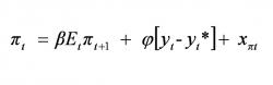
Equation 3
where yt denotes current real spending (in IS equation) or current output (in Phillips curve), Etyt+1 denotes the expected future level of spending, yt* denotes capacity output, rt denotes real interest rate, r* denotes rate of return prevailing in the absence of demand shock, Rt denotes nominal interest rate, πt denotes current inflation, Etπt+1 denotes expected future inflation, xdt denotes demand shock, and xπt denotes inflation shock (Robert G. King 2000, p.45-54).
The new model more clearly shows the limitations of monetary policies. Robert G. King (2000, p.45-81) argues that the new IS/LM model has strong conclusions: since the real economy cannot deviate from its capacity for long periods of time, monetary authorities cannot substantially influence the real economy in the long run; they should instead focus on neutral policies targeting a capacity output level or long-run inflation level. Monetary authorities are strongly encouraged not to pursue substantial influence (such as expanding the economy beyond its capacity), but instead to take a neutral policy, such as the Taylor rule, focusing on keeping the economy at its sustainable level.
The new IS/LM model gives us innovative, but largely limited, conclusions compared to the beliefs under the initial IS/LM model. Are these conclusions really consistent with what is observed in the economy? The main purpose of this paper is to verify the limitations of monetary policies concluded by the new IS/LM model by statistically testing alternative hypotheses using U.S. data from the past 50 years. Our alternative hypotheses pertain relationships between real interest rates and other main variables the real economy, which is contradictive to implications of the new IS/LM model. If results are statistically significant, it is likely that monetary policies have substantial influence on the real economy, despite contrary conclusions of the new IS/LM model.
Alternative Hypotheses Hypothesis I
We have hypothesized that net exports would be negatively correlated to real interest rates. This hypothesis postulates that when a trade surplus occurs for any given fiscal year in the United States, it will be invested domestically. This additional injection of investment funds diminishes the money attracted through credit in the economy, thereby depressing interest rates. The IS/LM exposition of general equilibrium in the domestic money and goods markets excludes the balance-of-payments equilibrium when the economy engages in foreign trade under conditions of fixed foreign exchange rates.
This hypothesis is supported by Dwayne Wrightsman (1970, p.203-208). He has derived a new external equilibrium curve to determine the relation between interest rates and income and superimposes this curve onto the IS/LM framework. The newly derived external equilibrium condition is shown in Figure 1. The lower right-hand section of the diagram in Figure 1 illustrates that the net exports of goods and services vary inversely with the level of national income. The upper left-hand section in Figure 1 indicates that net foreign investment varies inversely with domestic interest rates. The lower left-hand section in Figure 1 shows a 45-degree line that represents the relation between net exports of goods and services and net foreign investment. These results in the curve are shown in the upper right-hand section in Figure 1, which represents the relation between income and interest rates. From these four sections of the diagram, we can find that an increase in net exports will decrease income (Y) as well as interest rates. In Wrightsman's model, when the net exports increase, the LM curve shifts to the right and achieves equilibrium if monetary and fiscal authorities do not intervene, leading to a decrease in interest rates. However, the government also plays an important role in deciding the equilibrium by policies causing a shock on the net exports, for example, by changing tariffs or changing government expenditure for exporting goods. If such policies cause a positive shock on net exports, shifting upward the curve in the lower right-hand section, this, in turn, shifts rightward the curve in the upper right-hand section, and vise versa.

Figure 1; External equilibrium curve to determine the relation between the interest rate and income - Note: The upper right-hand section shows a LM curve that represents a positive relationship between the national income (Y) and interest rates (r). The LM curve is deprived from the lower right-hand section, the lower left-hand section and the upper left-hand section. The lower right-hand section shows a negative relationship between income (Y) and net exports. The lower left-hand section shows a 45 degree line that represents a relationship between net exports and net foreign investments. The upper left-hand section shows a negative relationship between net foreign investments and income (Y).
Hypothesis II
We have hypothesized that if we lower the level of inflation in the United States, this would result in lower real interest rates in the country. David Wessel (1999, A1) supports this hypothesis. He has argued that a high rate of inflation could distort the financial markets; this would lead to uncertainty among investors and to undermine public faith in the government. This leads to consumers holding more money in fear of a financial collapse. If the inflation rate continues to increase, it would cause consumers to borrow additional funds from banks; since the loan depreciates over time, the result would be an increase in real interest rates. This argument implies that a lower level of real interest rates is achieved if the inflation rate is kept at a low level, which supports our hypothesis.
Kandel et al. (1996, p.205-225) provides a statistical argument to support our hypothesis. Contrary to predictions using some conventional theories, they have found no negative relationship between real interest rates and inflation during the low and stable inflation sub periods.
Wessel (1999, A1) also provides an argument in favor of our hypothesis. In his article "With Inflation Tamed, America Confronts an Unsettling Stability," Wessel has argued the negative effects of a no-inflation economy on employment. That is, a low inflation rate generates significant stability in the economy and attracts foreign investors confident in their positive financial results, thereby reducing employment. From the psychological perspective, workers must get used to raises that look small but are worth the same as previous years. More than that, some workers will feel even discomfort about the perceived insignificant increase in their salaries.
Wessel (1999, A1) has also argued possible links between no inflation and the economy. One possible negative link is that corporate sales will stagnate; thus, profits will not be boosted. Consequently, workers' wages may fall, their skills may no longer be needed, and more unemployment will be created. Another positive link is that, in a no inflation economy, unemployment may decrease as investments rise due to the stability of the economy, resulting in increased productivity. No inflation and economic stability result in increased government revenue, leading the government to reduce taxes. These tax cuts will enable corporations to enjoy more profits and revenues. A potential psychological effect would be that workers would consume more, since they do not prefer to have extra money in hand, rather than be concerned about the inflation level, as they are more likely to be during periods of hyperinflation.
In summary, all the abovementioned arguments not only support a significant relationship between lower real interest rates and lower inflation, but also expand the discussions to linkages between real interest rates and inflation rates to the real economy. This linkage is the purpose of our hypothesis, implying the possibility of monetary policies influencing the economy. However, this hypothesis is not supported by the new IS/LM model. The new IS/LM model concludes that a low inflation target policy will keep the economy activity at near capacity and real interest rates will move by reflecting changes in the output capacity. That is, if the capacity grows rapidly and inflation is controlled at a low level, the real interest rates will grow rapidly. Only if the capacity growth stagnates under a low inflation economy will the real interest rates also remain at a lower level, as our hypothesis predicts.
Hypothesis III
We have hypothesized that an increase in the real GDP will result in lower real interest rates along the IS curve. Many previous papers have discussed the monetary transmission mechanism,that is, the process through which monetary policy decisions are transmitted into changes in the real GDP. The mechanism starts with a monetary policy action on the short-run interest rate, which, in turn, has an effect on the long-term interest rate. This change in the long-run nominal interest rate in turn affects the real interest rate, resulting in a change in the real GDP. John B. Taylor suggests that the links of the monetary transmission actually form a circle that is closed by linking the movements in the real GDP back to the interest rate through reaction functions (J. Taylor 1995, p.151-171). In Robert G. King and Mark W. Watson's "Money, Prices, Interest Rate and the Business Cycle," the authors argue that the empirical results show a negative relationship between the real interest rate and the output (King and Watson 1996, p.35-53).
We have based Hypothesis III mainly on the work of Kurt Richebacher, whose article, "America's recovery is not what it seems," explains the main factors that have influenced the increase of the economy. Richebacher (2004, 34) has suggested a simple but vigorous conclusion: that the growth in the GDP in recent years was due to a significant jump in defense spending, which is a permanent, and possibly increasing, element for the United States economy since the country has been constantly involved in maintaining global peace and NATO functions. This increased defense spending caused an increase in the capital investment, which in turn increased the real non-residential fixed investment and the non-residential structures. While recognizing he has not yet seen the complete linkage in reality, Richebacher (2003, 34) continues his theoretical argument that the increase of the GDP causes more investments in the national infrastructure and lower taxes for the population as well as lets the government invest its financial resources in the private sector, which keeps real interest rates at lower level and leads to more profits in the economy.
A contradiction between our hypothesis and the new IS/LM is the sign of the correlation between the real GDP and the real interest rate. The forward-looking IS equation explains that, if growth of the current output capacity is combined with predictable continuing future growth of the output capacity, the current real interest rate also needs to grow. That is, both the real GDP and the real interest rate have a positive relationship.
From forward-looking IS equation (Robert G. King 2000, p.54-59.):
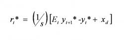
Equation 4
where * denotes that variables are at the capacity or sustainable level
This conclusion from the new IS/LM model is consistent with empirical results cited by King and Watson as mentioned earlier, but it is not consistent with Richebacjer's discussion. If our hypothesis shows significant results, we may assume a possibility of governmental policies stimulating the economy in such a way that the new IS/LM model does not predict.
Hypothesis IV
We have hypothesized that decreasing budget debt would result in lower levels of real interest rates. In the nation's fiscal outlook by the office of Management and budget, we see a high percentage of the budget deficit in the GDP.
The 2004 budget deficit came in at 3.6 percent of the GDP or $412 billion.
1. The 2005 deficit fell to 2.6 percent of the GDP or $318 billion.
2. The projected 2006 budget deficit would be at 3.2 percent of the GDP or $423 billion.
Covering the budget deficit could be achieved through the following means:
1. Increasing foreign investments in the United States economy; and
2. Increasing exports.
However, it is important to note that only the profit taxes and other fees left in the United States account for foreign investments; the rest goes to the investing country.
Any increases in exports that result in exceeding imports will have a positive impact; on the other hand, any decreased level in imports will have two effects:
1. It may lead to a decrease in consumption, which rarely happens, and result in increased savings due to the rise in interest rates; and
2. Consumers will have no choice but to purchase similar or substitute products, possibly national products, which ultimately will stabilize the level of consumption.
The second effect appears to be more realistic as it will lead to a decrease in the interest rate due to the increase of domestic private investments.
Our discussion considers complicated aspects, but it can be summarized in that countries with huge government debt/deficits discourage investments, force the nation to invite foreign investments, increase export/decrease import,which in turn pushes up the real interest rate,resulting in a reduction in the GDP.
On the other hand, the new IS/LM may explain the relationship between the government debt and the real interest rate using the forward-looking IS curve (Robert G. King 2000, p.54-59.):

Equation 5
In the new IS/LM model, the government deficit's influence on the economic activity is considered to be a negative aggregate demand shock (xdt less than 0), which may temporarily reduce the real interest rate but ultimately does not have a permanent influence on the output capacity, thus steadying the state real interest rate. If the government deficit is controlled at a lower level, the demand shock is mitigated and the economy returns to the steady state level. In other words, as mentioned during the discussions of the other hypotheses, lower levels of government debt or lower levels of demand shock do not result in lower levels of the real interest rate, which is decided by the expected future output capacity level and the current capacity level.
Our hypothesis challenges the new IS/LM conclusion about the influence of the government deficit on the real interest rate and economic activity.
MATERIALS AND METHODS
In the current study, we used vector autoregressions (VARs) and Granger Causality tests to verify the previous hypotheses. A VAR, introduced by Sims (1980), is an n-equation, n-variable linear model in which each variable is explained by its own lagged values plus lagged values of the remaining n-1 variables:

Equation 6
This simple framework provides a systematic way to capture dynamics in multiple time series and is easy to use and interpret (Stock and Watson 2002, p15.20-15.29). The Granger Causality test, developed by Granger (1969) and Sims (1972), is an F-test of the hypothesis that the coefficients on all values of one of the variables (xj,t-1, xj,t-2, . xj,t-q) are zero (H0: βj,1= βj,2=.= βj,q = 0) and xj is not a useful predictor given the other variables. In addition, impulse response functions (IRFs) of the VARs can be estimated to measure the effect over time on the variable of interest due to a change in other variable. Forecast error decomposition, the percentage variance of the error made in forecasting some variable due to a shock in a specific variable, complements the analysis by suggesting comparable degrees of interaction among variables (Stock and Watson 2001, p.101-115).
In the current study, we have assumed that the real economy would be influenced by many variables, such as real interest rates, inflation, and government expenditures, and that each variable would not only serially-correlated (correlated to its own past values) but also cross-correlated to other variables over time. Even in such a complicated situation, VARs and Granger Causality tests allow us to detect one-way or two-way relationships among many variables, avoiding misleading results caused by omitting variables. One concern was that we would need a large sample to test both tests holding many variables in a model. We have overcome this problem by collecting seasonally adjusted quarterly data, totaling over 180 observations, instead of yearly data.
The variables used in our models are real interest rates, inflation rate, real money supply, real GDP, real consumption, real investment, real net exports, real government deficit, which are included in the original IS/LM model or our hypotheses. Data are quarterly time series between the first quarter in 1959 and the last quarter in 2005, collected from Bureau of Labor Statistics (BLS), Federal Reserve System (FRS) and Bureau of Economic Analysis (BEA). Most of the data have been already seasonally adjusted, inflation adjusted and annualized. Otherwise, we have made the same adjustments on the unprocessed data. Economic time series are often analyzed after computing their logarithms or the changes in their logarithms since they are useful to capture the non-linear relationship and to measure elasticities (Stock and Watson 2002, p.15.5 -15.12). However, we did not use logarithms since we had many negative values in real interest rates and government deficit, for which logarithms could not be created. Instead, we used the percentage for real interest rates and directly calculated the percentage changes for the other variables.
For all the hypotheses, we tested VAR models with 1 through 12 lags in which real interest rates were regressed on the other variables:
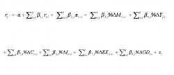
Equation 7
where q = 1, 2,., 12.
Additionally, in order to verify an extensional argument of each hypothesis, we tested models regressing net exports on the other variables for the first hypothesis, models regressing GDP on the other variables for the third hypothesis and models regressing the government deficit on the other variables for the last hypothesis. (See Table 1 for details.)
RESULTS
Models with shorter lags have not shown significant results in either Granger Causality tests or VARs. That is, Granger Causality tests have shown non-significant results at the 5% level (p-value less than 5 percent significant level) and VARs show little "fitting" (small R-square). However, the results have improved in models with longer lags while keeping the AIC from deteriorating (or increasing) compared to models with shorter lags. Therefore, in our analysis, we have mainly focused on the lag 12 model. (See Table 2).
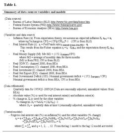
Table 1
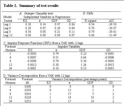
Table 2; Summary of test results - Note: EX denotes % change in real net export, π denotes inflation ratio (%), GDP denotes % change in real output, and GD denotes % change in real government deficit. The entries in panel A show the p-values for the Granger Causality tests testing the hypothesis that some variables are not predictable for real interest rates. The entries in panel C show responses in real interest rates. The entries in panel D show mean standard errors in forecasting real interest rates and Cholesky variance decomposition of the standard errors.
4.1 Hypothesis I
We tested the hypothesis that net exports negatively would relate to real interest rates (when EX↑, then r↓). The Granger Causality tests do not show that net exports are significantly predictive of real interest rates in a model with any lag. The VAR of the lag 12 model does not show constantly significantly negative coefficients of net exports. (See Table 3).

Table 3; Summary results for Hypothesis I - Note: the * in panel A denotes that the null hypothesis is rejected (predictive) at 10% significant level.

Figure 2a - Note: the solid line shows impulse responses in real interest rates over 24 quarters due to a change in net exports. 95% Confidence Intervals are given by the dot lines. The results are from a VAR with 12 lags. The scale is smaller compared to those in Figure 2b and 2c.
As a result, its IRF fluctuates around zero and does not continue to stay at either a negative level or a positive level over 24 quarters. (See Figure 2a.) In addition, its variance decomposition suggests that a shock in net exports causes very small responses in real interest rates. (See Table 1 and Figure 4b.)
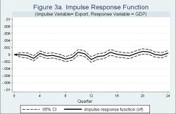
Figure 3a - Note: the solid line shows impulse responses in the real GDP over 24 quarters due to a change in real net exports. 95% Confidence Intervals are given by the dot lines. The results are from a VAR with 12 lags.
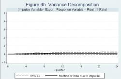
Figure 4b - Note: the solid line shows Cholesky variance decomposition (percentage points) of forecast errors, shown in Figure 4a, due to a change in real net exports. 95% Confidence Intervals are given by the dot lines.
On the other hand, the Granger Causality tests show that net exports are predictive of real GDP in the lag 12 model which is also implied in our hypothesis. (See Table 3.) However, its IRF also fluctuates around zero. (See Figure 3a.) Thus, the data suggests that exports are not consistently significantly predictive of real interest rates and GDP.
4.2. Hypothesis II
We tested the hypothesis that low inflation would brings down real interest rates (when low π, then low r). The Granger Causality tests show that inflation is significantly predictive of real interest rates in any model other than in models with lag 1 and lag 4. (See Table 4).

Table 4; Summary results for Hypothesis II - Note: the * in panel A denotes that the null hypothesis is rejected (predictive) at 10% significant level.
While the VARs of the lag 12 model do not show that the coefficients of inflation are constantly positive, its IRF remains at a positive level over 24 quarters. (See Figure 2b.) Therefore, the data suggests that inflation is significantly predictive of real interest rates, in addition, its signs of the reaction path are constantly positive over 24 quarters. Moreover, its variance decomposition indicates that a shock in inflation causes considerable responses in real interest rates. (See Table 1 and Figure 4c.) Low inflation does not seem to cause low interest rates. Looking at the time series graph, we do not find strong evidence that, when inflation is weak, the real interest rate is steady at a lower level. Whether inflation is weak or strong, the real interest rates fluctuate in almost the same way. (See Figure 5.)

Figure 2b - Note: the solid line shows impulse responses in real interest rates over 24 quarters due to a change in Inflation. 95% Confidence Intervals are given by the dot lines. The results are from a VAR with 12 lags.
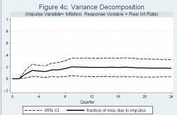
Figure 4c - Note: the solid line shows Cholesky variance decomposition (percentage points) of forecast errors, shown in Figure 4a, due to a change in Inflation. 95% Confidence Intervals are given by the dot lines.
4.3. Hypothesis III
We tested the hypothesis that the GDP negatively would relates to real interest rates (when the GDP↑, then r↓). The Granger Causality tests show the GDP to be predictive of real interest rates for models with 10 to 12 lags while its predictive power is not significant in models with shorter lags. (See Table 5). In addition, its variance decomposition suggests that a shock in inflation causes considerable responses in real interest rates. (See Table 1 and Figure 4d).
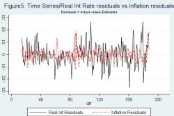
Figure 5 - Note: the "residuals" denote actual values minus estimated values from a VAR with 12 lags. The solid line shows "residuals" of real interest rates. The dot line shows "residuals" of Inflation. These lines represent the results between 1962 Q1 (13th quarter) and 2005 Q4 (188th quarter).

Figure 4d - Note: the solid line shows Cholesky variance decomposition (percentage points) of forecast errors, shown in Figure 4a, due to a change in the real GDP. 95% Confidence Intervals are given by the dot lines.
However, the VAR of the lag 12 model does not constantly show negative coefficients of exports. As a result, its IRF fluctuates around zero and tends to stay above zero over 24 quarters. (See Figure 2c).

Table 5; Summary results for Hypothesis III - Note: the * in panel A denotes that the null hypothesis is rejected (predictive) at 10% significant level.
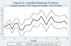
Figure 2c - Note: the solid line shows impulse responses in real interest rates over 24 quarters due to a change in the real GDP. 95% Confidence Intervals are given by the dot lines. The results are from a VAR with 12 lags.
On the other hand, the Granger Causality tests show that the GDP is predictive of investments in models with lag 1 and lag 8 while it is not predictive in the lag 12 model. (See Table 5.) However, the IRF shows investment's reaction against a GDP shock is initially positive but turns negative and finally fluctuates around zero over 24 quarters. (See Figure 3b).
Overall, there is no evidence of the hypothesis of negative predictive relationship between the GDP and real interest rates and the remaining part of our hypothesis regarding the positive predictive relationship between the GDP and investments.

Figure 3b - Note: the solid line shows impulse responses in real investments over 24 quarters due to a change in the real GDP. 95% Confidence Intervals are given by the dot lines. The results are from a VAR with 12 lags.
4.4. Hypothesis IV
We tested the hypothesis that the government deficit would positively relate to real interest rates (GD↑, then r↑). The Granger Causality tests indicate that the government deficit is predictive of real interest rates for models with 2 to 5 lags but its predictive power is weakened in models with longer lags. In addition, the VAR of the lag 12 model does not indicate that the coefficient of the government deficit is constantly and significantly negative. (See Table 6).
As a result, its IRF moves up and down around zero over time and does not show a tendency to remain either at a positive or negative level. (See Figure 2d.)

Table 6; Summary results for Hypothesis IV - Note: the * in panel A denotes that the null hypothesis is rejected (predictive) at 10% significant level.
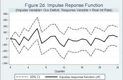
Figure 2d - Note: the solid line shows impulse responses in real interest rates over 24 quarters due to a change in the real government deficit. 95% Confidence Intervals are given by the dot lines. The results are from a VAR with 12 lags. The scale is smaller compared to those in Figure 2b and 2c.
In addition, its variance decomposition suggests that a shock in the government deficit causes comparatively very small responses in real interest rates. (See Table 1 and Figure 4e.)On the other hand, the Granger Causality tests indicate that the government deficit is significantly predictive of investments and the GDP in any model except for shorter lag models. (See Table 6). However, the IRFs fluctuate around zero and do not show a tendency to remain either positive or negative. (See Figure 3c and 3d).
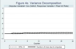
Figure 4e - Note: the solid line shows Cholesky variance decomposition (percentage points) of forecast errors, shown in Figure 4a, due to a change in the real government deficit. 95% Confidence Intervals are given by the dot lines.
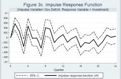
Figure 3c - Note: the solid line shows impulse responses in real investments over 24 quarters due to a change in the real government deficit. 95% Confidence Intervals are given by the dot lines. The results are from a VAR with 12 lags.
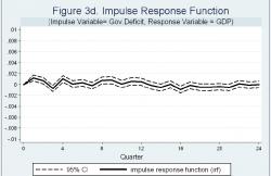
Figure 3d - Note: the solid line shows impulse responses in the real GDP over 24 quarters due to a change in the real government deficit. 95% Confidence Intervals are given by the dot lines. The results are from a VAR with 12 lags.

Figure 4a - Note: the figure shows mean squared errors over 24 quarters in forecasting real interest rates. The results are from a VAR with 12 lags.
Therefore, the data does not suggest a positively predictive relationship between the government deficit and real interest rates and the remaining parts of our hypothesis (i.e., IS/LM model's controversial argument that an increase in the government deficit crowds out investments, resulting in a reduction in the GDP).
DISCUSSION AND CONCLUSIONS
A major reason why the IS/LM model is useful and illuminating lies in the basic assumption of the model, which states that conditions of stock and flow equilibrium can be analytically separated. Tobin (1969, p. 16) found that "a key assumption is that spending decisions and portfolio decisions are independent,specifically that decisions about the accumulation of wealth are separable from decisions about its allocation. As savers, people decide how much to add to their wealth; as portfolio managers, they decide how to distribute variable assets and debts the net worth they already have." It should be recognized that the conditions under which such separation is valid are very stringent, and the assumption is probably a factor in the monetarist controversy.
Based on the study case presented, although government expenditures on defense and in other areas have been unprecedented compared to the previous century, the interest rates have been extremely low. Thus, it may be concluded that the factors that influence the interest rates are numerous and have different effects, both positive and negative. Although defense expenditures may lead to a sustainable percentage in the real GDP, it may happen, as presented in hypothesis IV, that the GDP is influenced by a budget deficit that keeps the interest rates at lower levels in order to encourage domestic private investments.
In analyzing the levels of the interest rates, it is better to look at the rate of inflation in the economy. A low inflation rate suggests that the economy is stable, which attracts investors to spend money in business and influences the interest rate in a downward direction in order to sustain these investors and attract the money of the households in the economic circuit through the banking system. The interest rate may also depend on the consumption culture. On the consumption side, the permanent income theory by Milton Friedman (1957) and the life-cycle theory by Modigliani and Richard Brumberg (1954) were developed within frameworks that emphasized the inter-temporal nature of household consumption decisions. If the population of a country is keener on spending money instead of saving it in a bank, interest rates will fall.
Another major factor of interest rate changes is the monetary policy of the government. For example, Mankiw, Miron, and Weil (1987, p358-374) show that the pricing of medium-term government bonds changed systematically with the introduction of a central bank in exactly the way predicted by the rational expectation theory of the term structure. When large, systematic changes in policy take place, then the tool of rational expectations gives a good account of how private responses will be altered. If a government "loosens" its monetary policy (prints more money), interest rates lower because more money is available for lenders and borrowers alike.
The new IS/LM model has provided an econometric specification, including a list of variables to be used in the regression equations and hypotheses about the magnitudes of effects to be used. In our analysis, we have also considered the important role the rational expectation plays and explored the effects of various frictions systematically. This could enable policy-makers and other macroeconomists not to depend too much on the traditional IS/LM model while contributing to subsequent research on this topic.
We started with the proposition that finding significant relations between the real interest rates and core variables in the economy could imply a possibility for monetary policies to overcome the limitations concluded by the new IS/LM model,that is, the possibility for monetary policies to influence the economy. We prepared four hypotheses involving relationships between the real interest rates and net exports, the GDP, inflation, and government deficit. Our hypotheses are alternatives to the new IS/LM model's conclusions. We then tested these hypotheses using U.S. data from the past 50 years according to the Granger Causality tests, the VARs and impulse response functions (IRFs). We have found from Granger causality tests that real interest rates would be predicted by the real GDP, inflation, or the real government deficit while they would not be predicted by the net exports. However, we have also found from IRFs that the predicted relationship would not be significant and consistent over time. Additionally, signs (positive or negative) in the relationships from Granger causality tests and IRFs would not necessarily be consistent with our alternative hypotheses. Another concern is that our tests used short-term interest rates. Therefore, significant results found in Granger causality tests may not contradict the new IS/LM model, which focuses on a long-run steady state. In addition, if our Granger causality tests have captured changes in capacity or steady state levels caused by past real interest rates, exports, inflation, or government deficits, our results might be explained by the new IS/LM model. In conclusion, our tests imply a possibility of overcoming limitations of monetary policies suggested by the new IS/LM model, but have not given us any conclusive answers. To find these, we need to conduct further research.
ACKNOWLEDGEMENTS
We wish to thank Professor Robert G. King, Professor Ani Dasgupta, Nicola Borri and Haizhen Lin at Boston University for comments and suggestions.
We are particularly indebted to our advisor Professor Ivan Fernandez-Val for his continued guidance and support.
REFERENCES
Berndt, Ernst R. "The Practice of Econometrics: Classic and Contemporary" MA: Addison Wesley, 1996.
Bruce, Neil "The IS-LM Model of Macroeconomic Equilibrium and the Monetarist Controversy" The Journal of Political Economy 85.5 (1977); 1049-1062.
Darby, Michael R. "The Financial and Tax Effects of Monetary Policy on Interest Rates" Economic Inquiry 13 (1976): 266-276.
Evans, Paul. "Interest Rates and Expected Future Budget Deficits in the United States" Journal of Political Economy 95 (1987): 34-58.
Fama, Eugene F. "Short Term Interest Rates as Predictors of Inflation" American Economic Review 65 (1975): 269-282.
Fama, Eugene F. and Gibbons Michael R. "Inflation, Real Returns, and Capital Investments" Journal of Monetary Economics 9 (1982): 297-323.
Fama, Eugene F. "Term-structure Forecasts of Interest Rates, Inflations, and Real Returns" Journal of Monetary Economics 25 (1990): 59-76.
Feldstein, Martin. "Inflation Income Taxes and the Rate of Interest: A Theoretical Analysis" American Economic Review 66 (1976): 809-820.
Fischer, Stanley. "Anticipation and the Nonneutrality of Money" Journal of Political Economy 87 (1979): 225-252.
Hoelscher, Gregory. "New Evidence on Deficits and Interest Rates" Journal of Money, Credit and Banking 18(1986): 1-17.
Huizinga, John and Mashkin, Fredric S. "Inflation and Real Interest Rates on Assets with Different Risk Characteristics" Journal of Finance 39 (1984): 699-712.
Kandel, Shmuel, Ahron R. Ofer, and Oded Sarig. "Real Interest Rates and Inflation: An Ex-AnteEmpirical Analyis" Journal of Finance 51 (1996): 205-225.
King, Robert G. and Mark W. Watson. "Money, prices, interest rates and the business cycle," The Review of Economics and Statistics, Vol.78, No.1 (1996): 35-53.
King, Robert G. "The New IS-LM Model: Language, Logic and Limits" FRB Richmond Economic Quarterly 86 (2000): 45-103.
Mankiw, N. Gregory, Jeffrey A. Miron and David A. Weil. "The Adjustment of Expectations to a Change in Regime: A Study of the Founding of the Federal Reserve," American Economic Review, American Economic Association, vol. 77(3) (1987): 358-74.
Mundell, Robert A. "Inflation and Real Interest Rate" Journal of Political Economy 71 (1963): 280-283.
Pennacchi, George G. "Identifying the Dynamics of Real Interest Rates and Inflation: Evidence Using Survey Data" Review of Financial Studies 4 (1991): 53-86
Plosser, Charles. "Government financing decisions and asset returns" Journal of Monetary Economics 9 (1982): 325-352
Richebacher, Kurt. "America's recovery is not what it seems" Financial Times 4 Sept. 2003: 34.
Riddell W. Craig and Smith Philip M. "Expected Inflation and Wage Changes in Canada, 1967-81" The Canadian Journal of Economics 15.3 (1982); 377-394.
Romer, David. "Advanced Macroeconomics" NY: McGraw-Hill, 2000.
Sparshott, Jeffrey. "American becomes global marketplace" The Washington Times 28 Dec. 2004: 15.
Stock, James H. and Mark W. Watson. "Vector Autoregressions" Journal of Economics Perspectives 15 (2001): 101-115.
Stock, James H. Stock and Mark W. Watson. "Forecasting Using Regressions with Time Series Data" handed in GRS EC542 Money and Financial Intermediation at Boston University in Spring 2006 (Draft 01/15/02) : 15-1 - 15-57.
Stulz, Rene M. "Interest Rates and Monetary Policy Uncertainty" Journal of Monetary Economics 17 (1986): 331-347.
Summers, Lawrence. "The Nonadjustment of Nominal Interest Rates: A Study of Fisher Effects" Macroeconomics, Prices and Quantities (Washington D.C., Brookings) (1983): 201-246.
Taylor, John B. "Monetary policy implications of greater fiscal discipline," Federal Reserve Bank of Kansas City (1995): 151-170.
Tobin, James. "Money and Economic Growth" Econometrica 33 (1965): 671-684
Tobin, James. "A general equilibrium approach to monetary theory", Journal of Money Credit and Banking, Vol 1, No 1 (1969): 15-29
Wachtel, Paul and John Young. "Deficit Announcements and Interest Rates" American Economic Review 77 (1987): 1007-1012.
Wessel, David. "With Inflation Tamed, America Confronts an Unsettling Stability" The Wall Street Journal 22 Feb. 1999: A1.
Wrightsman, Dwayne. "IS, LM, and External Equilibrium: A Graphical Analysis" American Economic Review 60.2 (1970); 203-08.